Climate-smart agriculture in Zambia
Average Marginal Effects
A model that speaks in log-odds is a model almost nobody can read. This is the translation step.
The Bayesian multinomial logit reports its results in log-odds. That is the right scale for the maths and close to useless for a reader, because almost nobody can look at a log-odds coefficient and say what it means for a farmer.
An average marginal effect is the translation. It asks: if you changed one thing about a household, by how much would the probability of it holding a given bundle of practices change? Then it answers in percentage points, which is a unit people can argue with.
The word average is carrying weight. The effect of a year more schooling is not the same for a household with two hectares and no credit as for one with twenty and a bank. So the calculation works out the change for every household in the sample, one at a time, and then averages across all of them. The result is the effect for the sample as a whole, not for some imaginary typical farmer who does not exist.
Because the model is Bayesian, this is done by simulation from the posterior rather than by a formula, which has the useful side effect that the uncertainty comes through with it.
What it cannot do
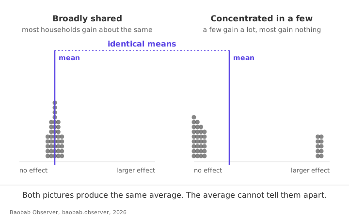
An average conceals its own spread. A marginal effect of two percentage points is consistent with two points for everybody, and it is equally consistent with ten points for a quarter of households and nothing at all for the rest. Those imply completely different policies and the average cannot tell them apart.
That is not a flaw so much as a division of labour. Finding out who the effect belongs to is what the causal forest is for.
The equation
AMEk = (1/n) Σi [ change in P(y = j | xi) when xk moves ]
- i
- each household in the sample, taken one at a time as itself
- xk
- the one thing being changed: a year of schooling, a hectare, credit or no credit
- P(y = j | xi)
- that household’s probability of ending up in bundle j
- (1/n) Σ
- and then the average across every household, rather than a calculation done once at the means
Computing it at the average household would be quicker and would describe nobody. This computes it for each real household and averages afterwards, which is the version that means something.
From the Zambia climate-smart agriculture research, built on the Water and Soil Accelerator household survey, which was funded by USAID. The thesis is under examination and the three papers drawn from it are under anonymous peer review, so there is nothing to link to yet.